• - (red) targets that were not directly traversed by an ion track,
• - (green) targets that were directly traversed once,
• - (blue) targets that were traversed more than once.
• Note that both f
1
and f
n
include contributions from δ-rays of nearby tracks.
• Substitute equation (2) into equation (1), and make the approximation that the
kernel function is constant for each of the microdosimetric components. The
resulting model is given by
• where
κ
0
,
κ
1
, and
κ
n
are free parameters quantifying the tumorigenic potential
of the three target populations.
• We also test the simplified 2-parameter model
• where
κ
01
is a free parameter accounting for both d
0
and d
1
target
populations.
(5)
(4)
(3)
(2)
(1)
Background
A Generalized Microdosimetric Dose Response Model
Shirin Rahmanian
1
, Tony C. Slaba
2
, Floriane Poignant
1
1
Analytical Mechanics Associates, Hampton, VA;
2
NASA Langley Research Center, Hampton, VA
• To ensure astronaut safety during and after deep
space missions, it is imperative to accurately
project radiation health risks.
• The current NASA cancer risk model relies on
dose-rate modifiers and radiation quality factors
(QF) to scale available epidemiological models
based on acute gamma ray exposures to the low
dose rates and complex mixed particle fields found
in space.
• QF models describe the increased biological
effectiveness of particles found in space compared
to gamma exposures and represent the major
source of uncertainty plaguing cancer risk
projections [1].
• Underlying these QF models are experimental
dose-response data obtained in cell cultures and
animals that provide a basis for estimating relative
biological effectiveness.
• As part of a broader effort to better understand and
reduce QF uncertainties, dose-response models
need to be improved and/or developed.
Objective
• In this work, a microdosimetric dose response
model is applied to the harderian gland (HG)
tumorigenesis experimental dataset [2].
• The model assumes that observed biological
responses should be correlated with, if not
predictable from, doses received by microscopic-
scale targets [3] (see Figure 1).
• To the authors knowledge, this microdosimetric
model has never been applied to the HG dataset.
• The performance of the microdosimetric model
against the HG data set was evaluated and
compared to a linear dose response model [2].
Optimal target
radius (µm)
Total number
of parameters
R
2
Akaike Information
Criterion (AIC)
Microdosimetric model (2 parameter*) 2.69 4 0.864 259.5
Microdosimetric model (3 parameter*) 2.67 5 0.865 261.3
Linear model** N/A 4 0.860 260.8
Modeling Methods
Results
Conclusions and Future Work
• The general form of the microdosimetric dose-response model is
Figure 1. Distribution of doses received by spherical targets
with radius 2.76
µ
m irradiated by 0.1 Gy of 600 MeV/n
56
Fe.
Table 1. Summary of model performance against HG tumorigenesis experimental data set for heavy ions only.
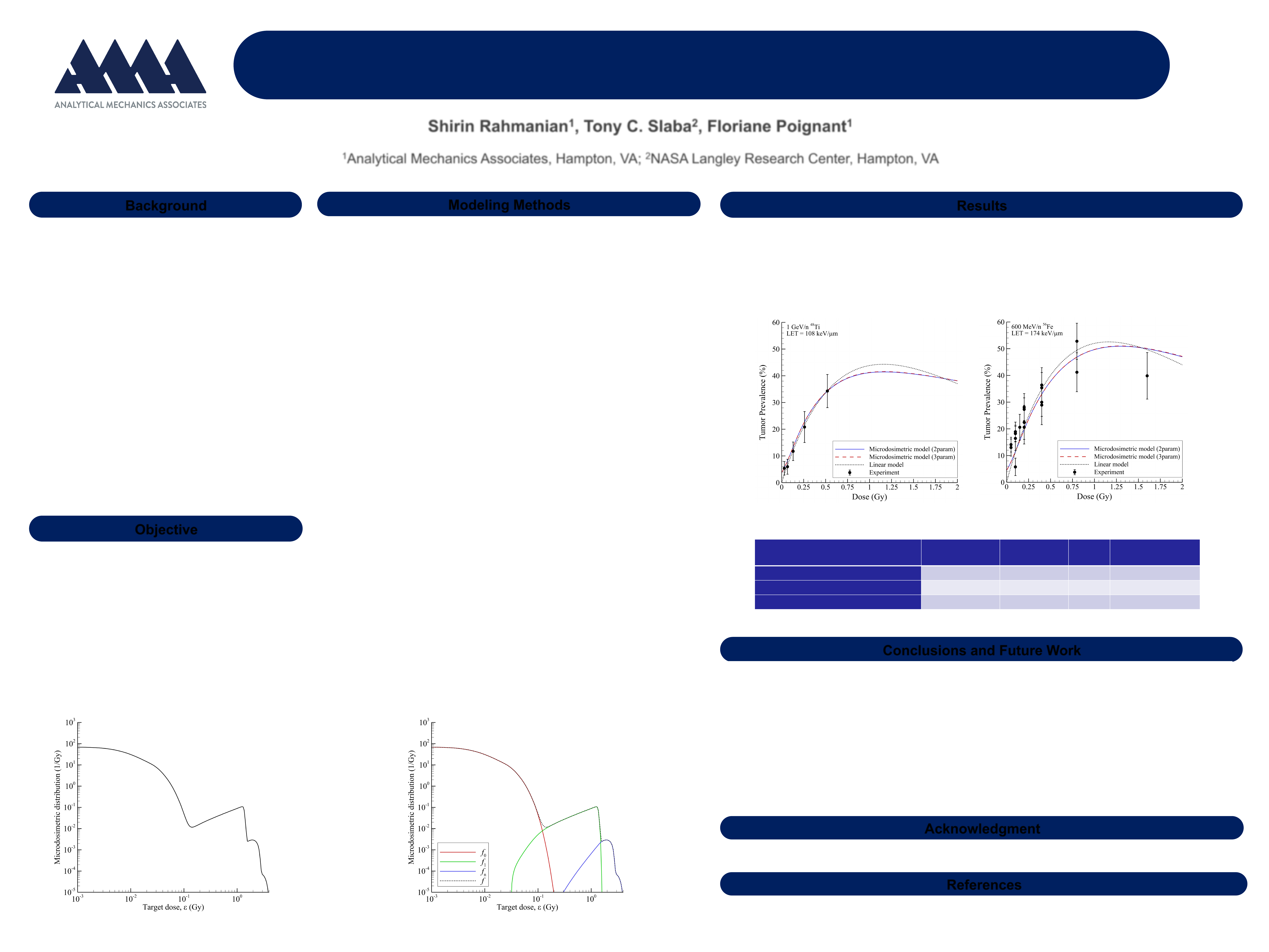
• A linear dose-response model from Chang et al. [2] is compared to the microdosimetric model in Figure 3
and Table 1.
• A high-dose attenuation term, e
-
α
D
, for cell killing/sterilization is applied as a multiplicative factor to all
models tested. The saturation coefficient, α, is treated as an adjustable parameter.
• The microdosimetric distributions are computed using RITRACKS [4] and convolution integrals [5].
• The microscopic target radius is also treated as an adjustable parameter (i.e. not fixed to 2.76 µm).
• Parameters are calibrated to available HG tumorigenesis experimental data for heavy ions [2].
• In this work, a microdosimetric dose response model was presented.
• The model relates observed biological responses to microscopic-scale spherical target doses.
• The optimal target radius was found to be very close to the HG nuclear radius of 2.76 µm.
• The microdosimetric model has a higher R
2
and lower AIC compared to the linear model.
• The microdosimetric model predicts charge and energy dependence of dose-response through the
biophysical spectra contained in equations (1) – (5).
• Ongoing and future work will include:
- Consideration of strictly numerical integral expansions including basis splines.
- Inclusion of empirical low-dose (non-targeted effects) corrections.
- Application of model to chromosome aberration datasets for fibroblasts and lymphocytes.
- Incorporate model into an ensemble framework with statistical weighting.
[1] Simonsen, Slaba, Life Sci. Space Res. 31: 14-28; 2021.
[2] Chang, Cucinotta, Bjornstad, Bakke, Rosen, Du, Fairchild, Cacao, Blakely, Rad. Res. 185: 449-460; 2016.
[3] Rossi, Zaider, Microdosimetry and its Applications, New York, Berlin, Germany, 1996.
[4] Plante, Cucinotta, in Application of Monte Carlo methods in biology, medicine and other fields of science, Rijeka, Croatia, InTechOpen, 2011, pp. 315-356.
[5] Kellerer, Chmelevsky, Radiat. Environ. Biophys. 12: 205-216; 1975.
References
Acknowledgment
This work is supported by the NASA Langley Research Center contract 80LARC23DA003 and by the Human Research Program under the Space Operations
Mission Directorate (SOMP) at NASA.
• P denotes the observed biological response (e.g. HG tumorigenesis)
• B denotes the collection of beam and target parameters.
o e.g. spherical target with radius 2.76 µm exposed to 0.1 Gy of 600 MeV/n
56
Fe, as in Figure 1.
• is the calculable microdosimetric distribution for spherical targets.
• is an unknown kernel function relating microscopic target doses to
observed biological responses.
( ) ()(; )P fd
BB
(; )f B
()
Microdosimetric Mod el
Bioph ysi cal Expansion
• The microdosimetric distribution, f, can be separated into biophysically
meaningful components (see Figure 2) according to
01
(; ) (; ) (; ) (; )
n
ff ff B BB B
0
(; )
f
B
(; )
n
f
B
1
(; )
f
B
Figure 2. Same as Figure 1, but the microdosimetric distribution, f,
has been separated into biophysically meaningful components.
00 11
() () () ()
nn
Pd d d BBB B
( ) ( ; ) ( 0, 1, )
ii
d f di n
BB
01 0 1
() [ () ()] ()
nn
P dd d
BBB
B
Figure 3. Comparison of models to experimental data for 1 GeV/n Ti (left) and 600 MeV/n Fe (right).
* Microdosimetric models include either 2 or 3 parameters along with the adjustable target radius and the saturation coefficient,
α
.
** The linear model [2] is given as P = (a+bLe
-cL
)De
-
α
D
, where a, b, c, and
α
are adjustable parameters, and L is the ion linear energy transfer (LET).
